Machine Learning for Engineers

1. Basic models

1.1. Regression

The goal is to estimate a function $( f(x) : y = X\beta )$ by minimizing the RSS (Residual Sum of Square):

L(\beta) = (y - X\beta)^T(y - X\beta)

Some assumptions:

Linearity: $( f(x) )$ is linear
Homoscedasticity: variance of residual is constant, check by plotting residuals vs x
Independence: all observations are independent of one another, check by Q-Q plot (see if sample quantiles vs the theoretical quantiles form a straight line)
Normality: distribution of Y is normal

1.2. Classification

Two types of classification models:

Generative models: These deal with the joint distribution of $( X )$ and $( Y )$ , then $( p(Y | X) = \frac{p(X, Y)}{p(X)} )$ . Examples include Naive Bayes, Gaussian Mixture Model, and Hidden Markov Model.
Discriminative models: These directly determine the decision boundary by choosing the class that maximizes the probability:

\hat{y} = \arg\max(p(Y = k | x))

1.2.1. Logistic Regression

Recall the sigmoid function:

S(X) = \frac{1}{1 + e^{-X\beta}}

The loss function for Logistic Regression, known as log-loss, is:

L(w) = \sum_{n=1}^N \left[ y_i \log \left( \frac{1}{S(X\beta)} \right) + (1 - y_i) \log \left( \frac{1}{1 - S(X\beta)} \right) \right]

In the case of more than two classes, softmax is used instead:

S(x_i) = \frac{e^{x_i}}{\sum_{j=1}^n e^{x_j}}

1.2.2. Decision Trees

For a discrete variable $( y )$ of $( k )$ states, the entropy is defined as the amount of uncertainty in $( y )$ :

H(y) = -\sum_{i=1}^k P(y = k) \log P(y = k)

Decision trees are learned in such a way that they maximize the information gain $( IG(Y, X) )$ :

IG(y, X) = H(y) - H(y|X)

Random forest is an ensemble of decision trees, where each is learned using bagging (both data and features), i.e., the tree is built only on a subset of data or features. XGBoost is another derivative of decision tree, where the estimators are different decision trees trained on the residual of the previous estimator successively.

1.3. Recommendation

Assuming that we can collect a huge matrix $( R(N \times M) )$ consisting of $( r_{i,j} )$ which is the relevance/rating of i-th user for j-th item.

User	Item 1	Item 2	...	...	...	Item M
User 1	$r_{1,1}$	$r_{1,2}$	...	...	...	$r_{1,M}$
User 2	$r_{2,1}$	$r_{2,2}$	...	...	...	$r_{2,M}$
...	...	...	...	...	...	...
User N	$r_{N,1}$	$r_{N,2}$	...	...	...	$r_{N,M}$

This matrix is extremely sparse as each user gets exposure to some among billions of items. The objective is to decompose $( R )$ into an user embedding matrix $( U \in \mathbb{R}^{N \times D} )$ and an item embedding matrix $( V \in \mathbb{R}^{N \times D} )$ such that:

\hat{R} = UV^T

Then, for any unseen item $( j' )$ in the matrix and any user $( i' )$ , the rating or relevance can be estimated as:

\hat{r}_{i',j'} = u'_i v'^T_j

There are several algorithms to matrix factorize, for example SGD (Stochastic Gradient Descent) or WALS (Weighted Alternating Least Squares).

1.4. Ranking

Ranking problems answer the question of given a query $( q_t )$ and a set of items $( U := \{u_i\} )$ , the model should output an ordered version of U. There are three common approaches for ranking: point-wise, pair-wise, and list-wise. While point-wise is straightforward as we will train a model to predict directly the likelihood of the relevant $( p_i )$ for $( u_i )$ to be ranked highest. The ranking is obtained by ordering $( p_i )$ in the end. This formulation is harder, as we do not need to estimate precisely the likelihood to get the ranking. Pair-wise instead formulates the problem to predict $( s_i := f(u_i) )$ and $( s_j := f(u_j) )$ for any pair $( (u_i, u_j) )$ . These two outputs are mapped to a learned probability that $( u_i )$ should be ranked higher than $( u_j )$ via a sigmoid function:

p_{ij} = P(u_i \succ u_j) = \frac{1}{1 + e^{-\sigma(s_i-s_j)}}

We then finally use the cross-entropy as the loss function to penalize the deviation of the model output probabilities from the ground truth. The whole learning to rank is assembled in a Siamese DNN.

2. Online and offline metrics

2.1. Loss functions

2.1.1. Classification

Cross entropy also called log-loss:

L_{CE} = -\frac{1}{N} \sum_{t=1}^N \log(p_t)

where:

p_t = \begin{cases} \hat{y}_t & \text{if } y_t = 1 \\ 1 - \hat{y}_t & \text{otherwise} \end{cases}

When there are M classes (M > 2):

L_{CE} = -\frac{1}{N} \sum_{t=1}^N \sum_{i=1}^M y_{i,t}\log(\hat{y}_{i,t})

Normalized cross entropy overcomes the constraint of cross-entropy loss by normalizing CE with the probability of the ground truth:

L_{NCE} = -\frac{L_{CE}}{-p\log(p) - (1 - p)\log(1 - p)}

where $( p = \sum_{t=1}^N y_t/N )$ .

Focal loss:

L_{FL} = -\frac{1}{N} \sum_{t=1}^N \alpha_i(1 - p_t)^\gamma \log (p_t)

where $( \alpha )$ is the weight to handle the data imbalance, and $( \gamma )$ controls the shape of the Focal loss’s curve. The higher the value of $( \gamma )$ , the lower the loss for well-classified examples, so we could turn the attention of the model more towards hard-to-classify examples. Having higher $( \gamma )$ extends the range in which an example receives low loss. When $( \gamma = 0 )$ , Focal loss becomes cross-entropy.

Hinge: not only penalizes misclassified samples but also correctly classifies ones that are within a margin from the decision boundary (example SVM):

p_t = \max (0, y_t - (1 - 2y_t) \hat{y}_t)

Kullback-Leiber measuring "how many bits of information we expect to lose":

L_{KL} = \sum_{t=1}^N \hat{y}_t (\log(\hat{y}_t) - \log(y_t))

2.1.2. Regression

Classical loss functions are MSE, MAE, and MAPE. MSE is easy to calculate derivative, penalizes large error, but then more sensitive to outliers. MAE or MAPE avoid mutual cancellation of positive/negative errors, easy to interpret, but fail to penalize large error. MAPE puts heavier penalty on negative errors ( $\hat{y} > y$ ), so it favors models that under-forecast than over-forecast.

Some other metrics:

R-squared which is the proportion of variation in the outcome that is explained by the predictor variables:

R^2 = 1 - \frac{RSS}{TSS} = 1 - \frac{\sum(\hat{y}_t - \bar{y})^2}{\sum(y_t - \bar{y})^2}

SMAPE: to overcome some problems of MAPE:

L_{SMAPE} = \frac{100}{N} \sum_{t=1}^N \frac{|\hat{y}_t - y_t|}{|y_t| + |\hat{y}_t|}

SMAPE becomes unstable when both true and predicted values are close to zero.

Huber: less sensitive to outliers than MSE as it treats error as square only inside an interval.

L_\delta = \begin{cases} 0.5 \times (y_t - \hat{y}_t)^2 & \text{if } |y_t - \hat{y}_t| < \delta \\ \delta \left( |y_t - \hat{y}_t| - 0.5 \delta \right) & \text{otherwise} \end{cases}

Quantile sometimes we value underestimation vs overestimation differently. Example, a model to predict food arrival time would penalize more overestimation rather than underestimation. Quantile loss can give more (or less) value to positive (or negative) error:

L = \sum_{y<p} \lambda \times |y - p| + \sum_{y \geq p} (1 - \lambda) \times |y - p|

where quantile loss becomes MAE when $( \lambda = 0.5 )$ .

2.2. Offline metrics

AUC Receiver Operating Characteristics (ROC) curve is a curve showing the relation between TP and FP rate (y- and x- axis correspondingly). AUC is the integral of this curve. The higher AUC, the better (random guess is of AUC = 0.5)
MAP Mean Average Precision is used to evaluate the ranking quality. To understand MAP, let first define the P@k (precision at k), which is simply the precision of k-most relevant items ordered by predicted relevance (or probability)(same definition for R@k - recall at k). Then, AP is defined as a metric that tells how much the relevant items are concentrated in the high ranked prediction, i.e.:

AP@K = \frac{1}{N} \sum_{k=1}^K P@k \times rel_k

where K is the number of items to recommend out of N items, and $( rel@k )$ is just an indicator that says whether k-th item is relevant (1 or 0). Now think of AP@K as a single data point. The quality of a recommender is measured as the average of every point till K:

MAP@K = \frac{1}{K} \sum_{k=1}^K AP@k

NDCG Normalized Discounted Cumulative Gain We start with the simplest metric, which is Cumulative Gain (CG). CG is essentially the number of relevant items recommended in the returned set:

CG@K = \sum_{1}^{K} rel_k

CG naively measures the quality of the recommendation by counting the number of relevant items being recommended. It is easy to interpret, but unchanged if the order of the set changes. A better metric is Discounted Cumulative Gain (DCG), which is defined as:

DCG@K = \sum_{1}^{K} \frac{rel_k - 1}{\log(k + 1)}

Then IDCG@k is defined as the best possible value for DCG@k, i.e., the value of best possible DCG where all $( rel_k )$ is set to 1. Finally:

NDCG@K = \frac{DCG@K}{IDCG@K}

As being normalized, NDCG can be used to assess the recommendation quality of size-varied sets.

2.3. Online metrics

CTR refers to the click ratio, which is usually used to measure the success of a marketing campaign.
Time spent per active user, on the other hand, helps to understand the engagement of the audience.
Satisfaction metrics can be used also are rate of dismissal or user survey response. All these metrics can’t be measured/optimized offline in the training and offline evaluation process. They can be only measured only after deploying models on a small portion of the traffic (A/B testing).

3. Feature Engineering

3.1. Encoding

One-hot encoding: common for categorical features of small and medium cardinality. However, tree-based algorithms do not perform well, especially at high depth. This is due to how the tree splits the data to maximize the information gain. If a feature contains many different values, splitting on any of this one-hot won’t give a significant IG, so tree-based algorithms tend to ignore these columns. Note that linear models don’t suffer from this problem.
Target encoding: Categorical features are replaced with a blend of posterior probability of the target given particular categorical value and the prior probability of the target over all the training data. In other words:

x_{cat_i} = \frac{1}{N_{cat_i}} \sum y_t|x_t = cat_i

Using the whole training data for target encoding will lead to label leakage. It’s important to apply additive smoothing or cross-validation.

Feature hashing: Categorical features are encoded to a higher dimensional space of integers, where the distance between two vectors of categorical variables is approximately maintained in the transformed numerical dimensional space. With Feature Hashing, the number of dimensions will be far less than the number of dimensions with simple One Hot Encoding.

x'_i = \text{hash}(x_i) \mod d

where d is predefined dimension of hash embedding.

Embedding learns a fixed-length representation of input features such that if $( x_i )$ and $( x_j )$ are related, $( d(e_i, e_j) )$ is also relatively small. There are two ways of learning embeddings: word2vec style and co-trained style. In the first style, training categorical features should appear in sequence like words in a sentence, for example sequence of users that a person reacts to, a sequence of stores one visits in the same browsing session. Denote ( x_t, t = 1, 2, ... ) are the categorical features we want to embed that appear in the same sequence. The embedding is learnt via a supervised task of predicting:

x_t = f (x_{t-1}, x_{t+1}, x_{t-2}, x_{t+2}, ...)

or:

x_{t-1}, x_{t+1}, x_{t-2}, x_{t+2}, ... = f(x_t)

In the co-training setup, embedding layers are plugged directly into any supervised neural network architecture. This is called neural embedding, or supervised embedding. StringLookup is first used to map the categorical features into integer indices with handling of unseen categories. Then Embedding layer is used, with learnable function activated to let the weights tuned during the supervised learning process as a whole.

3.2. Normalization and Standardization

For numerical features, we can use either normalization:

x'_{i,t} = \frac{x_{i,t} - \min(x_i)}{\max(x_i) - \min(x_i)}

or standardization:

x'_{i,t} = \frac{x_{i,t} - \bar{x}_i}{\sigma_i}

Outliers can cause severe problems in case of normalization, which can be fixed by using clipping where we pick a reasonable min and max values. If the feature distribution resembles power laws, we can use log-transformation:

x'_{i,t} = \log \left(1 + \frac{x_{i,t}}{1 + \text{median}(x_i)}\right)

4. Machine learning practices

4.1. Common DNN architectures

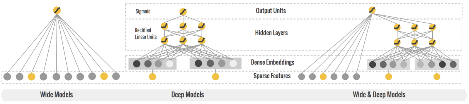
Deep-wide architecture: Deep network is successful thanks to its capabilities to learn and explore new and hidden features that appear less frequently in the data. Wide network, on the other hand, memorizes the frequent co-occurrence of features and explores the available correlation in the data. The Deep-wide architecture combines both benefits of these networks, and merging these features together improves model performance compared to DNN.

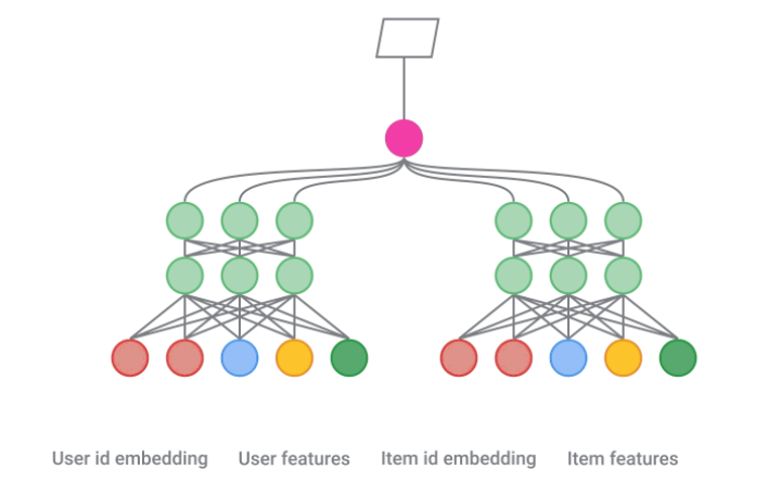
Deep-wide architecture. Source: https://ai.googleblog.com/

Two-tower architecture: Frequently used in recommendation, two-tower model is a common and effective pattern, which contains two sub-models that learn representations for queries and candidates separately. The score of a given query-candidate pair is simply the dot product of the outputs of these two towers.

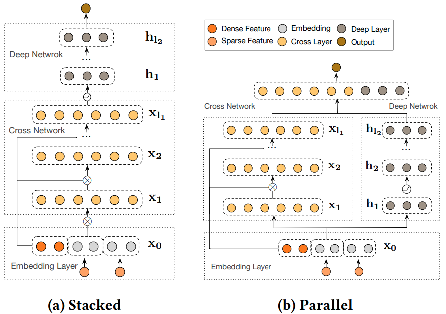
Two-tower architecture. Source: https://blog.tensorflow.org/

Deep Cross Network (DCN): Cross features are important in most applications to capture the patterns that appear across different features. However, it’s difficult to handcraft those cross features. Deep and Wide network can learn those combinations by memorizing from the data in the wide network. However, in practice, it’s difficult to pick which features to put in the wide network among thousands of available features. DCN was designed to explicitly and effectively learn cross features. It starts with an input layer (typically an embedding layer), followed by a cross network containing multiple cross layers that model explicit feature interactions, and then combines with a deep network that models implicit feature interactions.

Cross network explicitly applies feature crossing at each layer:

x_{i+1} = x_0 \cdot (W \times x_i + b) + x_i

The highest polynomial degree increases with layer depth. In practice, it’s best to use 2 cross layers.

Deep network contains traditional MLP layers. Cross network can be put in parallel to the deep network, or stack the deep network on top of the cross network.

Deep cross network: (a) Stacked, and (b) Parallel. Source: https://arxiv.org/pdf/2008.13535.pdf

Multi-task architecture: In many setups, the same set of features are used at different downstream tasks. Multi-task architecture helps to leverage the learned representation across different tasks. This setup is particularly interesting for recommendation, for example, as the same set of features are used to predict different reactions (like/comment), or different subset of recommendation.

4.2. A Facebook field guide to Machine Learning

Machine Learning Life Cycle. Source: https://research.facebook.com

Facebook Machine Learning team have developed a series of videos containing practical ideas and learning to help engineers and researches apply machine learning to real world problems, which includes six steps:

Problem definition
Data
Evaluation
Features
Model
Experimentation

4.2.1. Problem definition

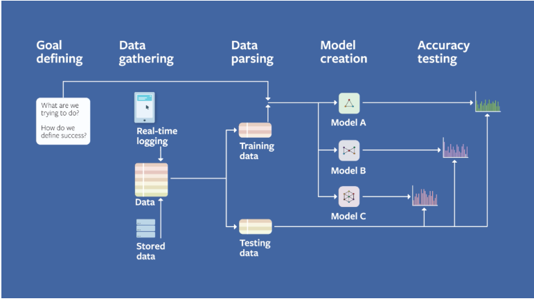
To bring Machine Learning to improve your product, it’s important to understand everything before and after deploying a model. The choice of the right setup is more important than the choice of the algorithm. To choose the right setup:

Choose the right Machine Learning task, from a business problem to which data, features, models, predictions, and how it improves the business performances.
Define how success looks like How to track user enjoyment/engagement, and how to monitor small changes in performances. To do so, we need to dig into the data to see if there are simpler tasks that can act as good proxies to your ultimate goal. The proxy event should:
- Happen in reasonably short period of time
- Not be too sparse/imbalanced
- Have features that contain predictive information about the proxy event.

4.2.2. Data

Data is the most powerful variable we can control to create a successful Machine Learning application. Data processing normally come in a form of joining different sources of information. There are 2 areas of data processing we should pay attention to:

Data recency and real-time training Data is rarely iid over time. It contains also seasonality. Models hence should be able to adapt to data distribution changes. A common practice is to train models until day N, and monitor performances at day N+1, N+2, ... If performances drop rapidly over time, it’s worth to invest engineering to have real time training. However, this requires real-time training data, which come with its own challenges:
- Real-time join is not efficient with batch querying system like Hive or Presto
- Delay between events cause inaccuracy in the training data (for example, delay between impressions and clicks)
- And online/offline inconsistency. For static features such as age, gender and location, we can easily recompute at training time. However, for time-dependent features, it’s better to use feature store, which cause extra storage cost and difficult to correctly version.
Records and sampling We need to be careful of systematic missing data due to logging, which require robust monitoring to detect. Importance sampling is the technique to help improving model performances and reduce training costs.

4.2.3. Evaluation

Evaluate offline, then online Offline evaluation, on the one hand, is fast, so it’s adapted to wide exploration. Online evaluation, on the other hand, gives richer information about the impact of a Machine Learning model to the business. It’s the key to perform offline evaluation until you have a viable candidate to validate with online experiments.

Create baseline models To do offline evaluation on a given test set, it is important to build a baseline model. The baseline aims at giving a context to all statistics we compute. A golden rule is to split data into train/validation/test sets. Random split has a danger of learning from recent data (hence, the future). A solution is to use progressive evaluation where we split the data in time. The choice of metrics is also important. Metrics should be interpretable and sensitive to model improvements. For example, AUC and R2 have their own baseline, while precision and recall lack of sensitivity in case of extreme imbalance.

Calibration of the model, defining as:

\text{Calibration} = \frac{P_{\text{predictions}}}{P_{\text{labels}}}

Calibration is a sanity check of model quality. Model should be calibrated on both training/test sets and online traffic:

Miscalibrated on training set implies model has not trained properly
Miscalibrated on test set implies model does not generalize well
Miscalibrated when model is online implies model online-offline gap

Miscalibration implies problem is usually fundamental. It makes sense to diagnose the model carefully.

Specificity and sparsity tradeoff The consideration of specificity is also important. For example, dataset can contains a large number of subset. The computed statistics is therefore weighted toward the largest subsets, which is somehow expected. However, it’s still useful to compute the statistics on different subset to understand where the performance comes from and whether it’s expected.

4.2.4. Features

In the feedback look among Data, Feature, Model and Evaluation, features are the second most important to model performance after data, but faster to iterate. Features should be relevant to the output and interpretable by the model. The choice of features should depend on model architecture, feature properties, special cases, and how much training data.

Derived features and feedback loop Apart from categorical and continuous features, derived features are very important to improve model performances. For example, historical CTR of an use is important to predict clicks. However, this feature makes it hard to interpret the output and hinders the generation of new hypothesis. Also, such derived features introduce feedback loop, which we need to be careful to understand and interpret the results.

Feature semantic changes We should be aware of feature semantic changes. Same definition of a feature should be agreed across different teams. Monitoring system should be in place to detect any outlier or dramatic shift in the feature distribution. If the semantics change, we should introduce a new feature to the model and eventually deprecate the old one instead of mixing together.

Feature leakage and coverage require also some attention. When the output is too good, there’s probably feature leakage. Feature coverage represents the percentage of missing data. Monitoring system should be robust to track feature coverage to ensure the health of our Machine Learning system.

4.2.5. Model

Ideally, data and features should decide which model to pick. To choose a good model, we should take into account:

Interpretability and ease to debug
Data volume
Training and prediction consideration

Linear model is a good choice in many situation as it’s interpretable, easy to debug, very fast at inference time, and work well with a wide range of data. For example, linear model works well when there’s few data and features. Large scale linear models work also extremely well when there are a lot of sparse features. Though in real life, most tasks respond in a nonlinear way, there are many strategies for capturing nonlinear interactions in linear model (for example cross features and embedding).

Calibration A good model should be well calibrated. One way to check is to split data into small groups (for example by ages/genders/locations) and check the calibration in each subset. As splitting to even small subsets will make calibration more difficult, this is still an indicator that the model is bias and need some treatment.

Model choice Data should influence the choice of models. Mature problems where a lot of data and compute power available will tend to favor Deep Learning. Problems with weak baseline and good intuitiveness will tend to favor more feature engineering with a simple model approaches.

Model setting Once the data and features are fixed, and a model is chosen, the task is to find a good choice of settings for this model. The settings can be broken down into hyper-parameter and model architecture.

Model versus infra costs The model in PRD is not always the one with best evaluation metrics. We also need to think about infra costs. Sometime, biggest gain comes from an increase in infra cost instead of data or features.

4.2.6. Experimentation

AB test For models like image and speech recognition, offline evaluation is representative of evaluation in real life. But it is not true for most other uses. If a model directly influences the dataset on which future iterations of it will be trained, we need different approach for experimentation. Key way to ensure similar behavior offline and online is absence of feedback loops. The key to ensure offline and online consistency is to isolate feedback loop using A/B test, where we split online flow of users into control and test groups. To make AB test more practical, we need to:

Minimize the time between hypothesis and first online experiment
Isolate engineering bugs from Machine Learning performance issues
Test model in the presence of real world feedback loop

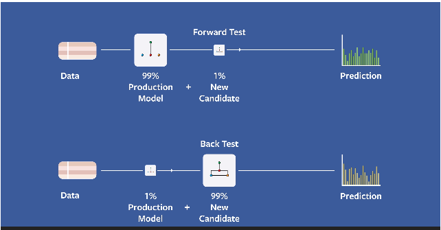
Feedback loop is unavoidable in real world applications. The contents we show today as a result of model A will become training data for model B. Forward and backward tests are used to validate a model in the presence of feedback loops. We forward test the model with 99% of users in control group with PRD model, and 1% in test group with the new model. In this case, the system feedback loop is dominated by the control group. After launching, we test 99% the traffic with new model and only 1% with old one. This will validate the size of the effects that were initially observed.

Machine learning model testing: Forward versus Backward test. Source: https://research.facebook.com

Measure any metrics we can Although we might be optimizing for one specific metric, measure as many meaningful metrics as possible. Most of the times, only few are important to prove our hypothesis, but others are useful to validate correctness of the experiment itself.

4.3. Steps to design a ML system

4.3.1. Project setup

Goal

This project aims at maximize/minimize ...
The system will be used by XXX users per day / minute, and expected to do YYY inference per day/minute
Constraints: trade-off performance vs speed, performance vs randomness of recommendation

Requirements

Training requirement: should model be retrained frequently
Evaluation: how can one tell the ML system is satisfactory
Personalization: should we train one generic model for all, or specialized ones

4.3.2. Data pipeline

Data availability Determine which data is available, how frequently to store/retrieve them

Features Which features are used to train the model

Feature engineering:

Crossed feature
Embedding for categorical features (one hot encoding, feature hashing)
Feature normalization/standardization for numerical feature

Data imbalance: naive resampling (training data only; validation and test data should be intact) or synthetic resampling (using SMOTE, but not as widely used)

Data storage and feature storage:

How much data/features are needed to retrain the model frequently (hot/cold data storage)
How to store: parquet, partitioned by date/time

4.3.3. Model

Choose the model

Discuss the choice from simple (high explainability) to more complex (high flexibility)
Discuss the baseline model: 3 levels, random, human and simple heuristic.

Settings Discuss how to scale up the hyper-parameter and architecture search using multiple GPUs

Offline metrics logloss/AUC vs RMSE/MAPE

Online metrics user enjoyment/engagement, revenue lift

Retrain requirement

Use a scheduler to retrain model on a regular basis (usually multiple time per day)
This frequency should be scheduled according our measure of online metrics.

4.3.4. Inference / Serving

Where and how to run inferencing: user device or server; at which latency; data privary

Retrain and fine-tune model:

Can we collect data from users to improve the model
If needed, add serving logic where requests will be sent to different models (for iOS/Android/Web...)
Track the online metric degradation to trigger model retraining
Compromise of exploration and exploitation: Thompson sampling

Scale Use an Aggregator Service to split the requests into multiple worker (similar to Load balancer)